The independent-samples t-test is conducted to compare two separate samples that are unrelated. The most common form would be a simple experiment in which a control group is compared to an experimental group.
For this next example let's pretend that there is a new method of math instruction that is predicted to be superior to older methods of instruction. We will form two equivalent groups of students by randomly assigning them to different classes. The control group will get the older, standard method of instruction. The experimental group will get the new instructional method. Both groups will be measured on a standardized math test at the end of the semester. The results will be compared to see if the new method is effective.
In PSPP, we will need two variables. The first variable represents the math scores (dependent variable). A second categorical variable is needed to code for the group membership, experimental or control. Here is what the data might look like in our example.
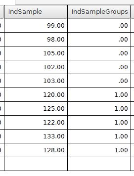
The variable IndSample is the dependent variable with the math test scores. The variable IndSampleGroups has a 0 or 1 coding scheme for representing the group membership. The 0 represents people in the control group. The 1 value is for people in the experimental group.
We will test for differences between the experimental group and the control group by using the independent-samples t-test. Choose the independent-samples t-test command by going to Analyze > Compare means > Independent Samples T Test. The following dialog box will be shown.
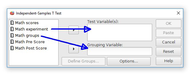
The first step is to choose the variables. Move the "math experiment" variable right to the Test Variable(s) field. This field is for the dependent variable. Move the "math groups" variable to the Grouping Variable field. This field represents the independent variable and group membership.
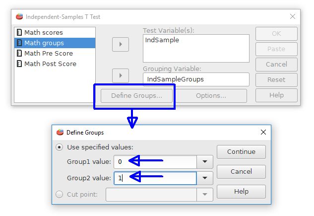
The second step is to inform PSPP how the groups are represented. Click on the Define Groups button. This opens a new dialog box. Enter the coding scheme values, which are 0 and 1 for our example. Note that PSPP has a feature for taking a continuously scaled variable and form two groups from a cutoff point if desired.
Press the Continue and OK buttons to perform the analysis. The output will look like this:
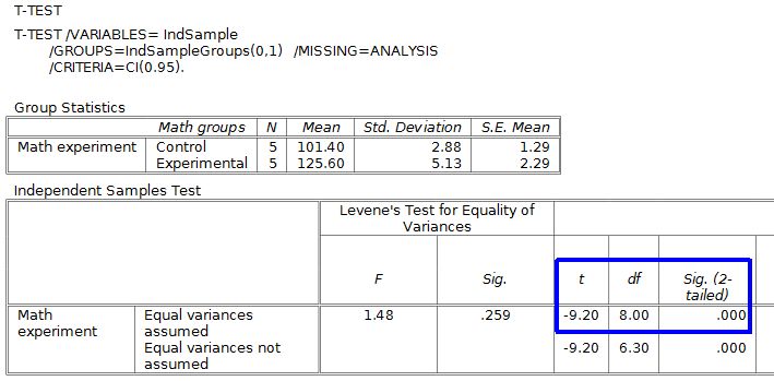
The upper table shows some useful descriptive statistics, like means and standard deviations.
The lower table has the t test results. This gets a little tricky because there are two versions of the test: Equal variances assumed and equal variances not assumed (see the rows). For most situations we will use the equal variances assumed version.
How can you tell which version to use? The Levene's test part of the output will give you the answer. When this test is nonsignificant use the equal variances assumed version. The Levene's test p value for this example is p = .259, so we will use the equal variances assumed version (marked in blue).
Our t-test result is t(8) = -9.20, p < .001 when expressed in APA style. We will reject the null hypothesis because this p value is less than .05. This is a statistically significant difference. The students who get the new math teaching approach are doing better than the students who received the older teaching approach.
Note that the p value (see Sig. 2-tailed) that PSPP gives is .000. Having a zero p value is not really possible, but PSPP can't make a judgment about something impossible. It would be best to report this result as p < .001 rather than p = .000.
A common mistake is to report the results from the Levene's test as being the t-test results. The Levene's test just helps us decide whether or not we need the equal variances assumed version of the independent-samples t-test. The Levene's test is not the actual t-test.
In regard to nomenclature, the equal variances version of the t-test is the classic Student's t-test. The unequal variances version is the Welch's t-test.
Home | Start | Variables | Data | Descriptive | Relationship | Inferential | Effect size | Advanced | Video
This work is licensed under a Creative Commons Attribution 4.0 International License that allows sharing, adapting, and remixing.